Tables, Equations, and Graphs: How to Move Between Three Forms of Linear Relationships

Imagine a ride-sharing trip with a $3.00 base fare and an additional $1.50 for every mile traveled. The total cost changes in a predictable way as the distance increases.

• The fares can be organized in a table to show the cost at different distances. 

• An equation could help us describe the pattern and calculate the fare for any number of miles. 

• We could use a graph to see the relationship visually and compare how quickly the fare increases. 

These may look like three different approaches, but they all show the same linear relationship in different forms. Each one gives us another way to understand the same real-world situation.

Today, we’ll learn how to represent linear relationships using tables, equations, and graphs. Then, we’ll explore how to move between these forms.

What Is a Linear Relationship?

A linear relationship connects two quantities that change at a steady rate. In other words, each time one quantity increases by the same amount, the other changes by the same amount too.

Think about renting a bike. You pay a fixed starting fee before you begin riding. Then, every extra hour adds the same charge, so the total cost increases at a steady rate.

To describe these two parts of the total, the starting fee and the steady increase, we use these math terms:

• Initial value, also called the constant term: This is the amount we start with. In our example, it’s the fixed starting fee.

• Rate of change, also known as the slope: This tells us how much the total changes each time the other quantity increases by one unit. In our bike example, it’s the charge for each hour.

We can represent the same linear relationship in three ways: with a table, an equation, or a graph. Next, we’ll see how our bike-rental example looks in each form.

A. Table

Suppose the bike rental starts at $3.00 and costs another $1.50 for each hour. A table pairs each number of hours, our input x, with the matching total cost, our output y:

B. Equation

An equation turns a linear relationship into a rule we can use for any input. 

For our bike rental, we can let x stand for the number of hours. The hourly part of the cost is 1.5x because each hour costs $1.50. This tells us how much we pay for the riding time.

We also need to include the $3.00 starting fee. So, we add 3:

1.5x + 3.

The total cost is our output (y) so the full equation is:

y = 1.5x + 3.

Here:

• x is the number of hours.

• y is the total cost.

• 1.5 is the rate of change, or slope.

• 3 is the initial value, or starting fee.

Our bike-rental equation follows the standard form of a linear relationship where y depends on x:

y = mx + b, where m is the rate of change, or slope, and b is the initial value, or the constant term.

C. Graph

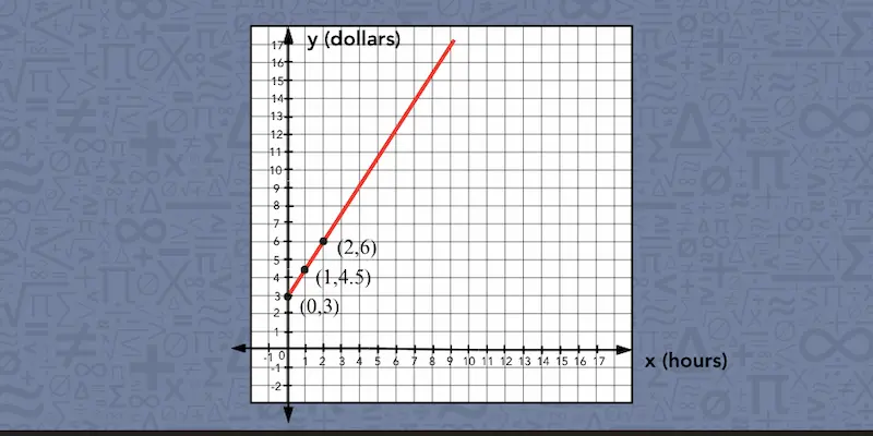
We can also plot the same input-output pairs on a graph, with hours on the x-axis and total cost on the y-axis.

For example:

• 0 hours matches with $3.00, so we plot (0, 3).

• 1 hour matches with $4.50, so we plot (1, 4.5).

• 2 hours matches with $6.00, so we plot (2, 6).

After that, we can connect the points with a straight line. In this situation, we only use values where x ≥ 0 because a bike rental cannot last a negative number of hours.

Now that we’ve seen the same relationship in all three forms, let’s find out how to move from one form to another.

How to Write an Equation From a Table of a Linear Relationship

To write an equation from a table, we follow these steps:

• Check that the values change at a steady rate. 

• Find the initial value.

• Find the rate of change.

• Put both into the standard form y = mx + b.

Let’s say your class is tracking money raised for an upcoming school field trip. The amounts collected each week are listed in a table.

The table gives us several matching values, but we want an equation that can predict the class budget for any week, even one that is not shown. To do that, we need to figure out how quickly the budget is changing and what amount it started with:

1. Check that the values change at a steady rate: From one row to the next, the week number goes up by 2, and the class budget goes up by $50. Since the same change happens each time, the relationship is linear.

2. Find the initial value: The table starts at week 2, so week 0 is not shown. We can work backward 2 weeks from $90. Because the budget changes by $50 every 2 weeks, we subtract $50: 90 - 50 = 40. So the initial value is $40.

3. Find the rate of change: The budget increases by $50 over 2 weeks, so we divide the change in y by the change in x: 50 ÷ 2 = 25. That means the budget grows by $25 per week. Notice that the slope is not 50, because the table moves forward by 2 weeks at a time.

4. Write and check the equation: Now we know m = 25 and b = 40, so the equation is y = 25x + 40. We can check whether the equation is correct by substituting values from one row of the table: 25(8) + 40 = 200 + 40 = 240. That matches the week 8 value, so our equation works. ✓

📕 You May Also Like: Functions vs. Equations: What Is the Difference?

How to Graph a Linear Relationship From an Equation

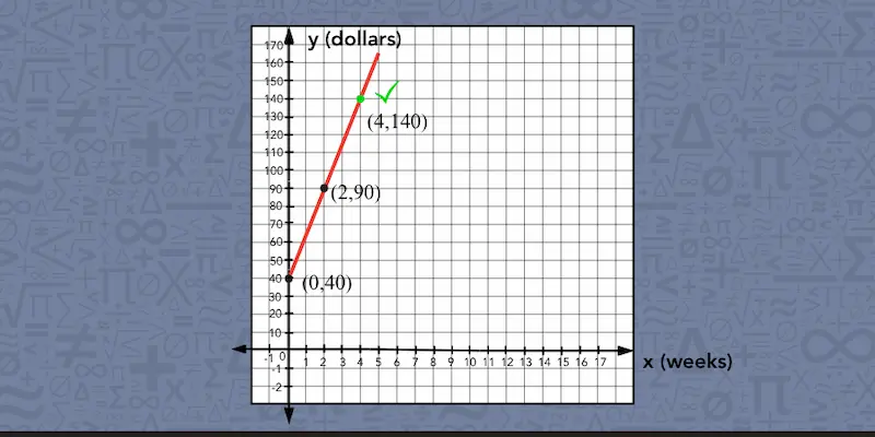
If we want to graph the equation, we can start with the initial value and then use the equation to find more points. For our class budget, the equation is y = 25x + 40.

1. Plot the initial value. As b = 40, we know that when x = 0, y = 25 × 0 + 40 = 40. So our first point is (0, 40), which represents a class budget of $40 at week 0.

2. Use the equation to find the next point. We can substitute different values for x and calculate the matching y-values. For example, when x = 1: y = 25(1) + 40 = 65. So we plot (1, 65). For x = 2: y = 25(2) + 40 = 90. That gives us another point, (2, 90).

3. Draw and label the line. As soon as we have several points, we can draw a straight line through them and label the axes: weeks on the x-axis and class budget on the y-axis. Since we are tracking time, we only use values where x ≥ 0.

4. Check one point. We can check the graph by choosing an x-value and using the equation to find the matching y-value. For example, when x = 4: y = 25(4) + 40 = 140. So the equation tells us that the point (4, 140) should lie on the line. We check the graph to make sure it does. If the line passes through (4, 140), our graph matches the equation.

📕 You May Also Like: How to Find the Slope of a Line—A Kid-Friendly Guide

How to Write an Equation and Make a Table From a Graph

When we have only a graph of a linear relationship and want to turn it into an equation and a table, we can work through these steps:

• Identify the initial value where the line crosses the y-axis. 

• Choose two clear points on the line and use them to find the rate of change. 

• Put the rate of change and initial value into y = mx + b.

• Use the graph or the equation to find matching x- and y-values for a table.

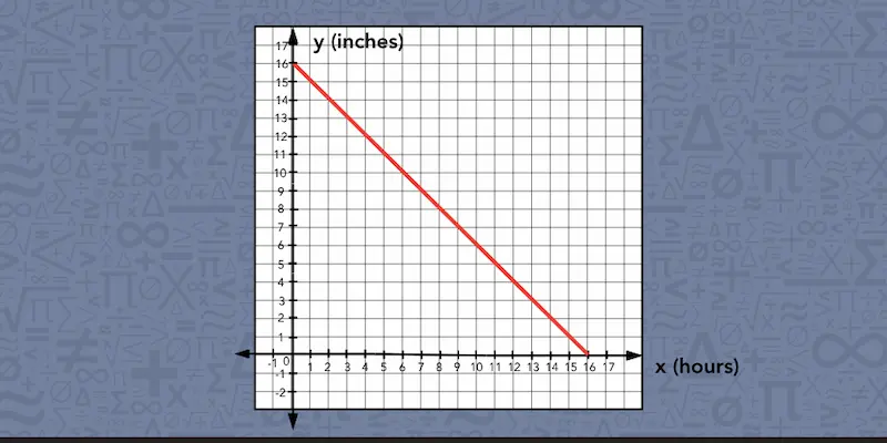
Now suppose we are given a graph that shows how the height of a candle, measured in inches, changes as it burns each hour. In this situation, we only use non-negative values because time cannot be negative. 

We also stop the graph when the candle reaches a height of 0 inches, since its height cannot keep decreasing below zero.

Let’s use what we can see on a graph to write the equation and build a table: 

1. Find the initial value. The line crosses the y-axis at (0, 16). That tells us that when x = 0, y = 16, so the candle starts at 16 inches tall.

2. Use two points to find the rate of change. Choose two clear points on the line, such as (2, 14) and (6, 10). From hour 2 to hour 6, x increases by 6 - 2 = 4, while y changes by 10 − 14 = −4. To find the rate of change, we divide the change in y by the change in x: −4 ÷ 4 = −1. So the slope is −1. The negative value tells us that the candle is getting shorter.

3. Write the equation. We know that m = −1 and b = 16. So we put those values into y = mx + b and get y = −x + 16. So this equation describes the candle’s height after x hours.

4. Build a table. Now we can choose different values for x and either read the matching heights from the graph or use the equation to calculate them. Here’s how the table looks like for our example.

📕 You May Also Like: What Is a Negative Slope? A Step-By-Step Guide

When Each Form Works Best for a Linear Relationship

Each representation of a linear relationship shows some details clearly and makes others less obvious, so the best form depends on the question we’re trying to answer. 

When a problem feels easier to understand in another form, you may try switching the representation. To help you decide which one to use, our tutors put together this table, showing what each form is especially useful for: 

📕 You May Also Like: How Multiple Representations Improve Understanding of Math

Try Showing This Linear Relationship in Different Formats

Practice switching between the formats yourself. For the relationship below:

1. Write the equation.

2. Graph it.

3. Use any form you like to find when the tank will be empty.

A water tank is draining at a steady rate. Here’s how much water is left after a few minutes:

You can check your answers at the bottom of the page.

Mathnasium tutors help students deepen their understanding of math concepts, such as linear relationships, by exploring them in different forms.

How Mathnasium Helps Students Connect Math Ideas (and Beyond)

Mathnasium is a math-only learning center dedicated to helping K–12 students of all skill levels excel in math.

When students come to us for math support, we focus on helping them understand how ideas relate instead of memorizing separate procedures. With linear relationships, that means seeing how a table, an equation, and a graph can all describe the same pattern in different ways.

To help students build that kind of understanding, we use the Mathnasium Method™, our proprietary teaching approach, to meet students where they are and guide them forward step by step.

Each student begins with a diagnostic assessment that helps us understand their current skill level, knowledge gaps, goals, and how they think and feel about math.

Using these insights, we create a personalized learning plan focused on the skills the student needs most, whether that means practicing operations with fractions and decimals, plotting points accurately, identifying rates of change, or preparing for more advanced algebra.

Our specially trained tutors follow the plan closely and provide live, face-to-face instruction in a caring and fun group environment. They use mental, verbal, visual, tactile, and written techniques to help students connect different representations of the same idea.

Students also get room to think through problems before tutors step in. Our tutors guide them to explain how different representations connect and check whether their reasoning makes sense. This helps students build critical thinking, problem-solving skills, and greater independence in math. 

Fun is part of the approach, too. We use game-based activities, rewards, and consistent encouragement to keep students engaged as they work with patterns, graphs, equations, and increasingly complex relationships.

The results? True, measurable progress:

• 94% of parents report an improvement in their child's math skills and understanding

• 93% of parents report their child's improved attitude toward math after attending Mathnasium

• 90% of students saw an improvement in their school grades

With over 1,100 learning centers across North America, there is likely a Mathnasium close to you.

For families in and near Mansfield, TX, Mathnasium of Mansfield North brings that same approach close to home, with specially trained tutors who help students make sense of tables, equations, graphs, and the algebra skills that connect them.

If your child needs support with linear relationships or any other math topic, a free diagnostic assessment is a great place to start. Using what we learn, we create a personalized learning plan that helps your child strengthen the skills they need next.

📅 Schedule a Free Assessment at Mathnasium of Mansfield North

Not near Mansfield?

📍 Find a Mathnasium Learning Center Near You

Pssst!... Check Your Answers Here

How did you do? Here’s how we can work through the draining tank example:

1. Equation. Each time x increases by 2, y decreases by 20, so the slope is −20 ÷ 2 = −10 gallons per minute. The table starts at 1 minute with 90 gallons. Since the tank loses 10 gallons each minute, at 0 minutes it had 90 + 10 = 100 gallons. With m = −10 and b = 100, the equation is:

y = −10x + 100.

We can check it with x =7: −10(7) + 100 = 30, which matches the table. ✓

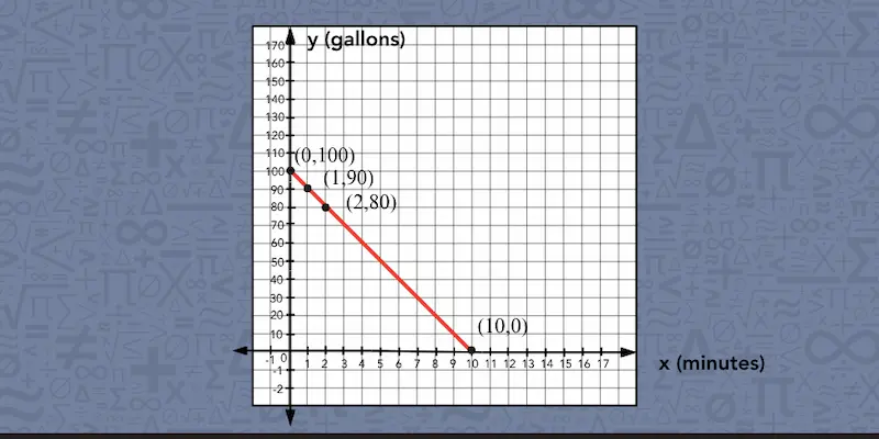
2. Graph. Start with (0, 100). Using the equation, we can find more points, such as (1, 90) and (2, 80), and draw a straight line through them. The line slopes downward because the amount of water decreases over time.

3. Empty tank. The tank is empty when y = 0: 0 = −10x + 100, so 10x = 100 and x = 10. The tank empties after 10 minutes, at the point (10, 0) on the graph.

Here, the graph only covers non-negative values because time and the amount of water in the tank cannot be below 0.